25 June, 2022

How To Use Decimal Places In Excel

To use Decimal Places in Excel, you will look at two buttons in the Number group of the Home tab Decrease Decimal and Increase Decimal -

You can utilize Increase Decimal after a number to increase the Decimal Places, similarly, if you want to clear the digits after the decimal from any number then you can utilize the Decrease Decimal button.

How to Automatically Insert Decimal Points in Excel

If you want that whatever data you enter in Excel will automatically get Decimal Points, then for this you have to

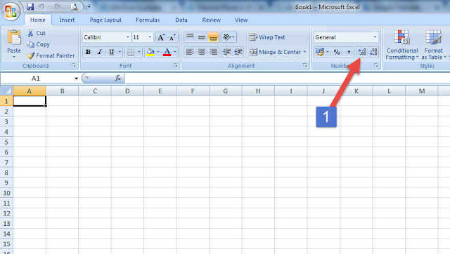
First of all, choose those cells in the Excel Sheet, in which you want to put Decimal Points Automatically.
You need to click on the icon given on the side of the Number group of the Home tab.
Here you will see the type in Number Tab in Format Cells.

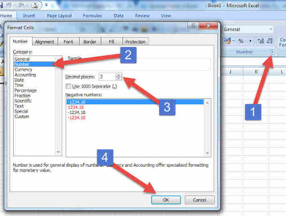
Here you need to choose the number, as soon as you select the number
You will find the option of Decimal Places, here you select Decimal Places and click on OK.

Find and Replace in Excel

Find and Replace in Excel:-

Keyboard shortcuts are there to find the text or number written in any cell in Excel. Ctrl + F will open a dialog box, here the search box will appear.

Type the text or number you need to look through in Find What
To look through Text or Number across the whole exercise manual or across sheets, select Workbook from the menu inside the Within the dropdown
Directly click on Find Next button to search through one by one.
To search through all text or numbers on the double, click on Find All

Now if you want to replace the found text, then click on Replace Tab.
Here you need to change that word in Find what
In Replace With, type the word with which you need to supplant the old word.
After this, if you want to replace only one word, then press the Replace button and if you want to replace all the words at once, then click on Replace All button.

Data Filter in Excel -

To filter the data in Excel, first select the header of the table.
Now go to the Editing tab in the Home Menu, click on the Short & Filter option here
Now select Filter in the menu, the Icon of Funnel is made on the Filter.

As soon as you select Filter, a menu will open on the header of your table, Text Filter will be given below, with this Text Filter you can filter your data.

Now you have to do this, if you want to filter the data from any text, only keep ticking it in the menu, from the rest of the text and remove the tick from Select All.

Sort The Data In Excel

Sort The Data In Excel:-

To sort the data in Excel, first select the table.

Now click on Sort & Filter option.
Here you will find two options if you have numbers in your table.

Sort Smallest To Largest
Sort Largest To Smallest

Similarly, if you have text data in your table then you should

Sort A to Z
Sort Z to A Two options will appear

Just choose the option in whichever way you like to sort
The whole table will be sorted according to whose column you will enjoy and sort.

18 June, 2022

Data Validation in Excel -

To use Data Validation in Excel, first select your table.
Go to the Data Tab, here you will see the option of Data Validation, click on it

Clicking on it will open the dialog box

In this dialog box, you will see 3 tabs Settings, Input Message, Error Alert
In the Settings tab, you have to set Data Validation Formula, with this you can create a drop-down list in any cell.
The other two tabs Input Message and Error Alert let you tell the operator what to type in the cell.
If Data Validation is installed in the cell and if someone tries to type it wrong then it will not be able to do it.

How to Change Case and Round Figure in Excel

How to Change Case

To change the case in Excel, type this formula in the cell in front of the cell in which you want to convert the text written in UPPERCASE -
=upper(cell name)
Suppose you have typed study skills in cell A1 and you want to convert it to UPPERCASE then you have to type
=upper(A1)
Similarly, to convert text to lowercase in Excel, you have to type this formula
=lower(cell name)
=lower(A1)

How to Round Figures in Excel

Suppose you have a 30.75 figure in an A1 cell and you want to convert it to Round Figures then you have to type Formula for this
=Round(A1,0)
By doing this, the digits after the decimal, if it is less than 50, then this result will be 30 and if it is more than 50 then the result will be 31.

How to make pivot table in excel

How to make a pivot table in excel?

To make a Pivot Table, first select the table or cell that you want to use in the Pivot Table.
After that go to the Insert tab and click on PivotTable
By doing this the dialog box of Create PivotTable will open.
Here you will find many options
Here you just have to choose a new worksheet or a Current worksheet in the location if you want to Existing
If you select the worksheet, then the Pivot Table will be ready on the same worksheet on which you are working.
On doing ok a blank PivotTable and Field List will be visible to you.
Now as soon as you click on the field, your PivotTable will be ready.

Uses of a pivot table

Uses of a pivot table:-

A pivot table helps users answer business questions with the tiniest step. Common pivot table uses include:

To calculate sums or averages in business concerns. For example, counting sales by unit or area.
To show totals as a percentage of a whole. For example, comparing sales for a detailed product to total sales.
To develop a list of unique values. For example, showing which states or countries have ordered a product.
To make a 2x2 table summary of a complex report.
To determine the maximum and minimum values of a dataset.
To query data directly from an online analytical processing (OLAP) server.

What is a pivot table?

A pivot table is a measurement device that sums up and rearranges selected columns and rows of information in a calculation sheet or data set table to get an ideal report. The device doesn't really change the accounting sheet or data set itself, it basically "pivots" or turns the information to see it according to alternate points of view.

Pivot tables are particularly valuable with a lot of information that would be tedious to calculate by hand. A couple of information processing functions a pivot table can perform include identifying sums, averages, ranges, or outliers. The table then, at that point, organizes this data in a basic, significant format that causes to notice key qualities.

How pivot tables work:-

When users create a pivot table, there are four main components:

Columns- When a field is chosen for the column area, only the unique values of the field are listed across the top.
Rows- When a field is chosen for the row area, it populates as the first column. Similar to the columns, all row labels are unique values, and duplicates are removed.
Values- Each value is kept in a pivot table cell and displays the summarized information. The most common values are sum, average, minimum, and maximum.
Filters- Filters apply a calculation or restriction to the entire table.

Create Data Entry Form in Excel Without Knowing Visual Basic

Create Data Entry Form in Excel Without Knowing Visual Basic

To make a Data Entry Form in Excel, you must first go to Office Button
Here you will find Excel options, click on it
Go to Customize here When you click on Customize, you will see a Drop Down Menu, in this Drop Down menu select Command not in the ribbon
Now below you will see a list, scrolling through it find the form,
When the options of the form are found, select it with the mouse and add it and click OK.
By doing this, the Options of the Form will be added to the Quick Access Toolbar of Excel.
Now design the data header of whatever data entry you want to enter in Excel.
That is, which columns you have to keep in that table like name, address etc.
Now just choose the Data header and click on the Options of the Form in the Quick Access Toolbar, a Dialogue Box will appear in front of you, OK it.
Then after, the Data Entry Form will be ready in front of you, you can extremely easily do Data Entry in Excel using this Data Entry Form,

How to Add a Word to the Beginning and Last of a Cell in Excel

In whichever cell you want to add any text to the beginning of the text written, then you have to type a small formula, suppose you want to add the text "Mr" to the beginning of "Ali" written in the A1 cell, then you have to type

= "Mr" & A1

Here you should also keep in mind that you have to give a space in front of whatever word you are adding like "Mr". You do not have to type "Mr".

If a name is written in A1 and the father's name is written in A2 and you want to combine both the cells like A1 and A2 then you have to type

="Mr"&B2 & "Son of Mr" &C2

So in this way you can combine the text written in two different columns.

Excel Camera amazing Tool | How to Use Excel Camera

Presently we should discuss the camera device of excel, when you have a lot of databases on excel, and there are many sheets and you need to show the main information of that large number of seats in a single seat then this camera device is exceptionally helpful. With this, you can undoubtedly deal with the information of all seats on any one seat and make a dashboard.

To activate the Excel Camera Tool, open MS Excel and go to the Office button, here you will see the Excel choice, click on it, in the Excel choice, you will see the choice of Customize, click on this likewise, you will see a rundown in Customize Here you need to choose all commands starting from the drop menu, a menu of many devices will open before you, from this menu you need to choose the camera and add it when you add the camera instrument from here. It will be shown in the Quick Access Toolbar of your Excel, in this way you can enact the Camera Tool in Excel.

Presently to show any cell with the help of a camera, first you select the cell, after that click ap on the symbol of the camera, presently any place you need to bring it from it, click it, then a picture of your cell is second. The place will come yet it won't just be a picture, at whatever point you roll out any improvement in the fundamental cell or change the information, however, it will likewise be a picture automatically,

5 Most Used Excel Formulas - If, Sumif, Countif, Vlookup,

1) if the formula excel -

The syntax of the IF function is as follows:-
IF(logical_test, [value_if_true], [value_if_false])

2) Sumif formula excel -

If there is such a list in your excel file, there is an item which is written more than once and you have to sum the number written in front of it, then this formula is needed like if you make a bill and anyone item in it If there is more than once then it can calculate the amount written in front of it in one go

The syntax of sumif function is as follows:-
SUMIF (range, criteria, [sum_range])

3) Countif formula excel -

The countif formula is used to account for any number or any name occurring more than once in any list in Excel.

The syntax of countif function is as follows:-
COUNTIF (range, criteria)

4) Vlookup formula excel -

Found on V Lookup is used in Excel when you have to search vertically for a particular value or lookup value.

The syntax of the Vlookup function is as follows:-
VLOOKUP (lookup_value, table_array, col_index_num, [range_lookup])

5) Vlookup formula excel -

The match function is used to define the position of any given name or value in the table, although this formula is very short, when mixed with other formulas, it becomes a very strong formula.

The syntax of MATCH function is as follows:-
MATCH(lookup_value, lookup_array, [match_type])